
We had a need to simulate beam propagation on our optics bench as a part of designing a new vortex trap, so I took to coding some of that up this weekend. Then, when I was most of the way through, I thought, why not build a UI and then other people could use it too?

The bundled-up EXE file [V2.0] is here, running it will extract the files to the current folder. But to then run the actual program you need the MATLAB compiler (MCR), so here‘s a version with it packaged in (caution: 300MB) if you don’t have that on your computer. If anyone wants the MATLAB code that went into it, here’s the link to that, also. The compiled code works on Windows 64-bit or 32-bit machines. But the pure MATLAB code is likely to run in any recent version of MATLAB.
This is just V1.0. And it’s very limited because I only implemented the optical elements that we needed- lenses, axicons, wave plates, apertures, etc. Also, I’ve done almost no optimization of the code, so the calculations are always done on an N x N grid with edge length D (N and D are set by the user). This software can’t really handle microscope applications, since 100x reduction in spot size requires resizing and resampling and though I’ve added a resample feature, you have to be fairly sparing about using it because the interpolation scheme works poorly when phase oscillations are rapid, so you’ll see artifacts sometimes. When I make improvements to the code, and I will before I release it to the group, I’ll update here too.
Update 1: I made wavelength an input parameter. Also I added tools for zooming in and out on the beam. [V1.1]
Update 2: Added Setup panel for user-specified resolution and edge length. Fixed the lag on calculating vortex wave plate element. Fixed some other bugs. [V1.2]
Update 3: Made window resizeable and open up smaller. Added image resampling and resizing. [V2.0]
Instructions:
The idea is pretty simple, the center panel always displays the beam profile at the plane of reference. The plane of reference is automatically set by the last optical element you added plus whatever propagation distance you specified behind it. You can undo your last step with the undo button. Or you can back the simulation all the way up to the initial beam by hitting start over. The history window displays all the manipulations done to the beam. It’s there so you can visualize the set up you’ve made so far.
- Enter the Setup information. Wavelength, Range, and Resolution. Range defines the box size for analysis, and is the length of one of the sides of the square. Default is 6mm. You want to choose a range that is large enough to accommodate any intermediate spot size in your optical path. Resolution is the number of pixels on a side. Default is 2048. Larger resolution takes up more ram and takes longer to compute.
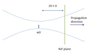
- To initiate the beam, create a gaussian beam. Gaussian beams are defined by 2 parameters. Here, I’m choosing the parameters to be beam waist (w0) and distance to waist (z0). I’m assuming you’re working with a laser here so beam waist ~1mm, and distance to waist is the distance from your reference plane to the narrowest point of the beam (the focus). E.g. Say you want to make a (nearly) collimated gaussian beam with radius of 1.5mm. Enter 1.5 and 0. Say you want to make a converging beam, you want to choose a positive waist distance, so you can try .4 and 500. Diverging beams have negative waist distance.
- Choose an optical element or propagate the beam forward to the next reference plane.
- Lens: focal length of lens (fl), distance to propagate after lens (z).
- Aperture: usually you want to add an aperture if you’re not certain that your lens or objective can catch all the rays from the beam, this way diffraction from an aperture is taken into account. Input: radius of aperture (r0), and distance to propagate after aperture (z).
- Axicon: creates a bessel beam. Input: opening angle (g), distance to propagate after axicon (z).
- Wave Plate: creates optical vortex. Input: topological charge (l), distance to propagate after waveplate (z).
- Propagation: this just propagates the beam by z. In other words, only moves reference plane forward or backward. Z can be positive or negative.
- Add more optical elements, apply “undo” liberally, examine the beam profile by moving reference frame forward and back. When you are happy with the beam you’ve created, copy down the elements you’ve added in the History panel.
- Any time you change the fields in the Setup panel, you want to hit the Start Over button to avoid errors.
- If your beam is becoming too large for the program’s field of view, resample and increase the range. Decrease the range if there is a lot of black space and you are losing detail. You can also add resolution, but most processors can’t handle much more than 4096 points on a side. Caution: resampling introduces artifacts, only resample if absolutely necessary and if the beam is not too divergent.

Example:
This is an example of creating a Bessel beam (using an axicon with g=0.5 degrees) and then reducing its size by 1/2 by a set of two lenses.

This is what it looks like when modeled by my application (V1.0).

Math notes:
Paraxial approximation throughout. Beam is propagated using the Fourier transform of the Fresnel kernel. If your beam exceeds the size of the computation region (that is, it does not go to zero at the boundaries), weird FT artifacts will start showing up with periodic repeating structure. If you see that, you need to reduce your beam size so it fits within the calculated area. There’s no ray tracing in any of this. I don’t really know how to do ray tracing…
